Set embeddings and anitag2vec
Problem statement
Given a finite collection of sets $C = \{ S_1, S_2, …, S_n \}$ , find a function that embeds the features of $S_k$ such that for sets $S_i$ and $S_j$ to have equal features, we require $f(S_i) = f(S_j)$.
In practical terms, such function $f$ would return a vector of dimension $N$ and we replace the equality constraint with the cosine similarity.
A tag embedding from scratch: anitag2vec
An interesting use-case is for tags (or hashtags) used in social medias, video/art sharing platforms, or even image sharing boards.
Without loss of generality, let’s focus on anime titles or artwork style tags found in websites such as Sakugabooru, Danbooru, Pixiv, or MAL.
Just like sets, order doesn’t matter: the embedding model must be permutation invariant to a certain degree.
Unlike vanilla sets in which we do not assume relationships between the members, tags are way more well-behaved. Some group of tags are more likely to be found together (e.g. #sketch #rkgk, #1girl #yuruyuri #bait).
Concept
Fundamentally, creating embeddings for a list of tags is about mapping an unordered set of items into a $N$ dimensional vector.
The task is quite similar to what Deep Sets paper do:
$$ M: T \rightarrow \mathbb{R} ^ N $$
with function/model $M$ to be permutation invariant
$$ M(T) = \phi_2 (\sum_{t \in T} {\phi_1 (t)}) $$
Which sounds reasonable but the issue is that most tags will have various spellings such as 1girl ~ 女の子 ~ girl, meaning you’d still have to group similar items somehow (I suppose you can use a dedicated word embedding for that task but that gives us another dependency).
anitag2vec assumes a simple transformer encoder architecture. We can also drop positional encoding since order doesn’t really matter as we mainly care about how each tag correlates/attends to each other within the set.
For the token embeddings, I use a BPE for the simple reason that it is fast to compute, and easy to configure.
Training and loss function
The signal lies in the data distribution itself, which means we can train in a self-supervised manner.
As for the loss, I use contrastive learning discussed in Representation Learning with Contrastive Predictive Coding paper and explored in InfoNCE paper.
The model implements 2 ideas:
IDEA 1. Permutation invariance:
We let the model learn about permutation invariance by augmenting the dataset with random permutations of each of its elements.
# This is an utility class for loading the data from a file
class MergeSet:
  # ...
  def extend_with_synthetic(self, perm_limit=5, sub_array_count=5) -> List[List[str]]:
      extended = []
      for example in self.real_examples:
          extended.append(example)
          if len(example) > 2:
              perms = 0
              for p in permutations(example):
                  extended.append(list(p))
                  perms += 1
                  if perms >= perm_limit:
                      break
              for _ in range(sub_array_count):
                  start = random.randint(0, len(example) - 2)
                  length = random.randint(2, len(example) - start)
                  sub = example[start : start + length]
                  random.shuffle(sub)
                  extended.append(sub)

      return extended
IDEA 2. Context relevance as objective:
The idea is that within a batch $B$, the model outputs
$$O \leftarrow M(B)$$
We then determine how each sample’s matching output distribution ressembles the others within that batch i.e. compute the self-similarity of the output.
$$ S := \text{norm } \{O \} \cdot \text{norm } \{ O \}^T $$ giving a square matrix of dimension $size(B) \times size(B) $.
For example $S[i][j]$ encodes exactly how much the i-th sample ressembles the j-th sample within the batch.
Our target is $\text{diag } S$, and it will all be just a bunch of 1s since at some position $k$, $S[k][k]$ is exactly how much the k-th sample ressembles to itself.
The trick is to augment the dataset by having two versions with each having some of its elements hidden, so to reformulate we have
$$O_{1} \leftarrow M(\text{aug_rand }B)$$
and,
$$O_{2} \leftarrow M(\text{aug_rand }B)$$
This results in a new similarity matrix:
$$S := \text{norm } \{O_1 \} \cdot \text{norm } \{ O_2 \}^T$$
In principle for any sample $k$, we want $S[k][k]$ to go towards $1$ which is similar at heart to having it “predict” the hidden tokens. To be more precise, the objective is to make diagonal similarities large relative to off-diagonal ones.
# ...
def augment_tags(x, drop_prob=0.15, shuffle=True):
    mask = torch.bernoulli(torch.full(x.shape, 1 - drop_prob)).to(x.device)
    x_augmented = x * mask.long()
    if shuffle:
        for i in range(x_augmented.size(0)):
            perm = torch.randperm(x_augmented.size(1))
            x_augmented[i] = x_augmented[i][perm]
    return x_augmented
This is optimized using a cross-entropy loss over the logits derived from the similarity matrix $S$. To emphasize stronger values, we will also introduce a parameter $\tau$ for the temperature.
$$ \text{logits} = S / \tau $$
$$ p_{ij} = { { \exp(\text{logits }[i][j]) } \over { \sum_{k=0}^{B-1} \exp(\text{logits }[i][k]) } } $$
$$ \text{loss}[i] = \sum_{j=0}^{B-1} -y_{ij}\log p_{ij} $$
But since the target $y_i$ is one-hot at index $i$ ($y_{ij} = 1$ if $i = j$ otherwise $0$), then
$$\text{loss}[i] = -\log p_{ii}$$
$$ \text{ce_loss} = {1 \over B} \sum_{i=0}^{B-1} \text{loss}[i] $$
def compute_loss(model, batch_data, temperature=0.07):
    o1 = augment_tags(batch_data)
    o2 = augment_tags(batch_data)
    o1 = F.normalize(model(o1), p=2, dim=1)
    o2 = F.normalize(model(o2), p=2, dim=1)
    logits = (o1 @ o2.T) / temperature
    loss = F.cross_entropy(         # !
        logits,
        torch.arange(o1.size(0)) # classes [0, 1, .., B-1]
    )
    return loss
This means that each row is trained to maximize probability to the diagonal entry. For each embedding in $O_1$, we identify its correct counterpart in $O_2$ among all batch elements. And simultaneously, all other entries in the row act as negatives.
A perfectly random model would produce $p = 1/B \implies \text{loss} = -\log (1/B) = \log B$.
In our case, for a batch size of $256$, if our the loss is higher than $\log 256 \approx 5.545$ then we are definitely doing something wrong.
python .\src\train.py
Training hash 896b40b1cf682c44, hyper parameter hash 63fc21b89723d1ce_b0d065e705028cb3
Loading tokenizer from './checkpoints/token_dataset_b0d065e705028cb3_vocab_size_5000_freq_3.json'..
Cooking model with 1,871,744 parameters
Loaded 196043 total examples | Hash b0d065e705028cb3
Splits: training 157043, eval 20000, test 19000
Batch size 256
Mean total Loss: 0.1288: 100%|█████████████████████| 15/15 [52:18<00:00, 209.21s/it]
Running tests
Training losses:
    0.42  ┤
    0.37  ┼╮
    0.33  ┤│
    0.28  ┤│
    0.23  ┤╰╮
    0.18  ┤ ╰────╮
    0.13  ┤      ╰───────
Here after 15 epochs, we jitter around $\approx 0.1288$, meaning our model is confident about the correct class about $87.91 \% $ of the time on average.
$$loss = 0.1288 = -\log p \implies p = \exp(-loss)= \exp(-0.1288) = 0.8791$$
This is quite strong since the task is 256-way discrimination, to put in perspective a random guess has $0.39 \%$ confidence rate on average.
For a sanity check to see if our model actually learns something useful, we will split the dataset into 3.
- $80 \%$ for the training.
- $10 \%$ for the evaluation split, for every epoch, we calculate this in order to see which hyperparameter the model performed best (mainly epoch in our case).
- And $10 \%$ for the testing split, this simulates real usage as it collects all the remaining data the model has never seen.
Here is what I got:
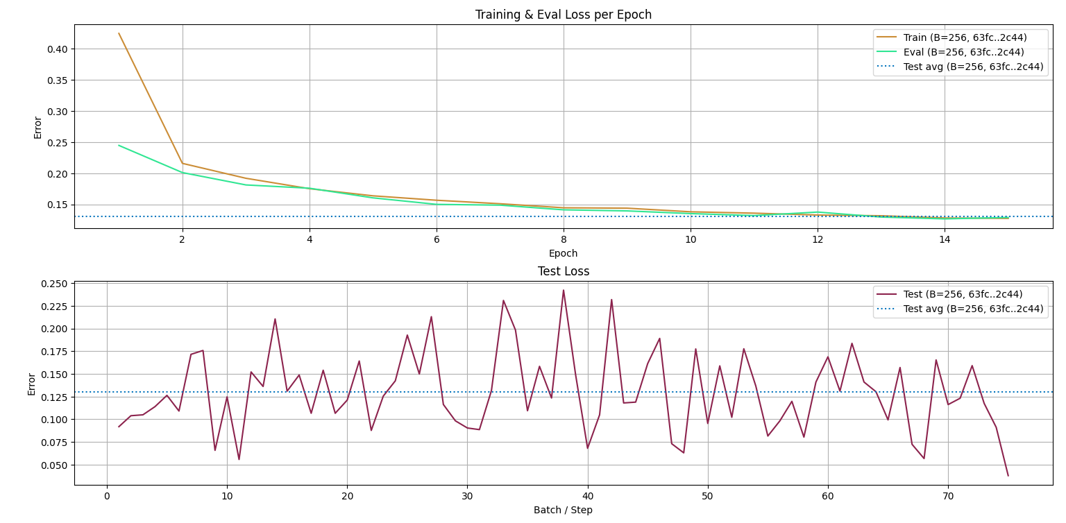
The first plot compares the training loss and evaluation loss, as you can see they both follow similar trend, no explosion in sight, nothing wrong here. The dashed line is the average test split loss, it meets the training loss at epoch 14/15-ish so we can assume the best model sits around that parameter. This also suggests we could have trained longer.
The second plot compares the test losses to its own average, it jitters around $\mu = 0.125 \pm 0.1$. Suggesting at best it will perform with $\exp(-0.025) \approx 97.53 \%$ confidence, and at worst $\exp(-0.215) \approx 80.65 \%$ confidence.
Architecture
A full implementation from training to inference is available at michael-0acf4/anitag2vec.
Input
The input is a batch of tags, we then encode these into token IDs. The number of tokens is unknown however, so we are forced to clamp when in excess or pad in scarcity. In any case, the input tensor dimension has to be fixed and we clamp/pad relative to that.
Basically, our model is a function taking $(B, I)$ and returning $(B, O)$. $B$ represents the batch dimension which we will omit for simplicity’s sake.
Embedding Layer (LUT)
This is a trainable lookup table with the goal of letting the model learn about the the tokens. It is required to be at least of the size of the vocabulary or the number of possible token IDs, or to be general, it has to be big enough for us to be able to address all the token ids.
In a nutshell, it receives the token IDs from the tags, then each token ID will map to the associated learned token embedding. In our case, the embedding output is a vector of dimension $D$, so for $I$ tokens we get $(I, D)$ shaped tensor.
$$ (I) \xrightarrow[]{\text {Embedding LUT}} (I, D) $$
Transformer encoder
The task of this layer is to determine the hidden relationship between the tokens. It receives the token embeddings looked up from the previous layer. I will not discuss how or why it works here but I’ve already made this and this a while ago if you are interested in the internals.
The key point to undersdand is that it is multi-headed, meaning for a given parameter $N$, we split the computation into $N$ parallel attention heads via leanred linear projections. Each head operates on a smaller subspace of dimension $D / N$, producing its own queries, keys and values. They all compute attention independently over the input sequence, and their outputs are concatenated along the embedding dimension, followed by a final linear projection.
For each head, we do
$$ Head_i = Attention(Q_i, K_i, V_i) = softmax(\frac {Q_i . K_i^T} {\sqrt {D / N}} + Mask) . V_i $$
But since we are encoder only, it reduces into self-attention i.e. $Q_i$, $K_i$, $V_i$ are all trained from the same source, the token embeddings of the input.
$$ Q_i = X W_{Q_i}, K_i = X W_{K_i}, V_i = X W_{V_i} $$ with $X \in \R^{I \times D}$ being the token embedding of the current tag set and $W_{Q_i} \in \R^{D \times D/N}$, $W_{K_i} \in \R^{D \times D/N}$ and $V_{V_i} \in \R^{D \times D/N}$ representing the weights the model improves from training. This makes $Q_i$, $K_i$, and $V_i$ to be of dimension $(I, D / N)$.
We will be setting $Mask = 0$; I did try masking on the transformer and the pooling layers only to have the model perform worse with the same configurations. After some trials, I reasoned that the $[PAD]$ token was still meaningful internally as it is being used to hide the tokens during the augmentation phase explained above, so we let the model understand what it means.
A linear projection is learned during this process, the input is the concatenated attention head results, and its forward pass is what we want.
Dimension-wise we get:
$$ (I, D) \xrightarrow[]{split} \bigoplus_{i=1}^{N} (I, D /N) \xrightarrow[]{N \text{ attention heads}} \bigoplus_{i=1}^{N} (I, D /N) \xrightarrow[]{linproj} (I, D) $$
Mean and Max pooling
The transformer output encodes how each token relates to each other. Its output contains contextual relationships and the target distribution itself. But our goal is to make a vector embedding i.e. we need to summarize that information into a configurable vector of size $O$.
- Mean: by averaging the transformer outputs accross the sequence, we extract the context contained within the current tag set.
- Max: similarly, we emphasize the most important features across tokens.
They each reduce a $(I, D)$ matrix into a $(1, D)$ matrix. And just like the idea used in the multi-head attention, we concatenate the results then have a trainable linear projection compress the information even further into our desired output dimension $O$.
$$ (I, D) \xrightarrow[mean]{max} (1, D + D) \xrightarrow[]{linproj} (1, O) \rightarrow (O) $$
Use-case example
This is the type of thing we can do:
Loading tokenizer from './checkpoints/token_vocab_size_5000_freq_3.json'..
Done!
Try an expression like "Drama, Romance, Supernatural" - 2 * "Shounen, TV"
You can also prefix the whole expression with ! to rank from worst
>>
>> "Comedy" - "Romance"
0.21: Cherry Teacher Sakura Naoki, Manga, Comedy, Ecchi, Shounen
0.2: Uramichi Oniisan, Manga, Life Lessons with Uramichi Oniisan, Comedy
0.19: Sunohara-sou no Kanrinin-san, Manga, Comedy, Ecchi

>> "Comedy" + "Romance"
0.65: Criminale!, Manga, Comedy, Romance
0.58: Mousou Telepathy, Manga, Comedy, Romance
0.57: Yawarakai Onna, Manga, Comedy, Romance
Cool right?
Computation Graph
                    batch of tags
                          |
                    [BPE encoder]
                          |
                 [batch of token ids]
                          |
                        (B, I)
                          |
                  [ Embedding LUT ]
                      (B, I, D)
                          |
    [  Transformer(d_model=D, nheads=.., nlayers=..)  ]
                      (B, I, D)
                     /         \
                    /           \
          [ Mean Pool ]         [ Max Pool ]
            context              highlight
            (B, D)                (B, D)
                     \         /
                     [   (+)   ]
                       (B, 2D)
                          |
                      [ Linear ]
                          |
                        (B, O)
Additional notes
Regarding the architecture, I figured this is enough:
# Hyper parameters
{
  "HYPERP_TAGTOK_MAX_TOKEN_CLAMP": 128,
  "HYPERP_TAGTOK_VOCAB_SIZE": 5000,
  "HYPERP_TAGTOK_MIN_FREQ": 3,
  "HYPERP_TRANSFORMER_D_MODEL": 128,
  "HYPERP_TRANSFORMER_N_HEADS": 8,
  "HYPERP_TRANSFORMER_N_LAYERS": 2,
  "HYPERP_OUTPUT_EMB": 128
}

# Training Config
{
  "TRAINING_EVAL_SPLIT": 20000,
  "TRAINING_TEST_SPLIT": 19000,
  "TRAINING_BATCH_SIZE": 256,
  "TRAINING_PERM_LIMIT": 8,
  "TRAINING_SUBARRAY_COUNT": 7,
  "TRAINING_SHUFFLE_SEED": 44276,
  "TRAINING_EPOCHS": 15,
  "TRAINING_LOGITS_TEMPERATURE": 0.07,
  "TRAINING_AUG_DROP_PROB": 0.3,
  "TRAINING_LEARNING_RATE": 0.0001
}
At the start, for the first samples we always get a loss around $\approx 5$. Interestingly, the average batch error quickly gets down to $\approx 1.5$ on the first epoch. For each configuration that I’ve experimented, I usually get about $100 \times$ to $200 \times$ confidence better than random. On the actual performance however, I noticed that quality is in the average loss decimals.
One thing to also note is that the batch size should scale relative to the permutation count and generated subarrays in order for the model to have more variety or ensure to have uniformly random batches at every iteration.